Physics and methods

What TreeLevel computes exactly, how, and against what it has been checked.

Contents

Scope
Conventions
Numerical amplitudes
Fermions: chains, signs, Majorana
Phase space and observables
Symbolic engine
Validations
Known limits

Scope

TreeLevel computes tree-level amplitudes (no loops), for initial and final states made of the model's elementary or effective particles: 2 → n scatterings and 1 → n decays. The results are cross sections in picobarns (partonic when quarks are involved: no parton distribution functions), partial widths in GeV, lifetimes in seconds (ħ = 6.582 × 10⁻²⁵ GeV·s), branching ratios when the model declares the total width. Declared resonance widths enter the propagators (−iMΓ in the denominator); the diagrams of a process are summed consistently, with their relative signs.

Conventions

Metric (+, −, −, −); ε⁰¹²³ = +1; γ⁵ = iγ⁰γ¹γ²γ³, P_L,R = (1 ∓ γ⁵)/2; Weyl (chiral) basis for the γ matrices, as in ALOHA.
Vertex rule = i × (Lagrangian term with the fields removed), all momenta incoming, ∂_μ → −i p_μ. Propagators: i/(p² − m² + iMΓ) for scalars, i(p̸ + m)/(p² − m² + iMΓ) for fermions, −i g^μν/(p² − M² + iMΓ) for vectors in Feynman gauge, with the −p^μp^ν/M² term in unitary gauge.
Standard Model: FeynRules conventions — D_μ = ∂_μ − i g_s T^aG^a − i (e/s_W) (σⁱ/2) Wⁱ − i (e/c_W) Y B, Φ = (−iG⁺, (v + h + iG⁰)/√2), Feynman–'t Hooft gauge; numerical parameters of the sm UFO (α⁻¹ = 127.9, G_F = 1.16637 × 10⁻⁵ GeV⁻², M_Z = 91.1876 GeV, M_W derived).
Colour: T^a = λ^a/2, standard f^abc, ε_ijk for triplets. External colour indices are summed, the initial state averaged (3 per quark, 8 per gluon).

Numerical amplitudes

At a given kinematic point, each diagram is a tensor network: the vertex rules (evaluated numerically with the legs' momenta), the propagators, and the colour deltas of the internal lines. The network is contracted over its internal indices in a greedy order (always the tensor sharing the most indices with the running result), which avoids forming large outer products — four-gluon vertices gain a factor 25. This network does not depend on the helicities: it is computed once, then contracted with the external wavefunctions (spinors u, v, ū, v̄ of helicity ±½; polarisation vectors ε^μ of helicity ±1, plus 0 for massive bosons) for each helicity configuration. Σ|ℳ|² is the sum over these configurations and over the external colours, divided by the spin and colour multiplicity of the initial state.

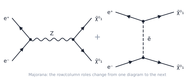
Diagrams whose external fermions play the same roles (row/column) share their wavefunctions: their networks are summed before the helicity loop. Integrations over angle or energy are spread over all cores.

Fermions: chains, signs, Majorana

Each continuous fermion line of a diagram forms a chain, read from the row spinor (outgoing ū or incoming v̄) to the column spinor (incoming u or outgoing v). The relative sign between diagrams is the parity of the permutation of the external fermions, and (−1) per fermion loop.

With Majorana fermions or fermion-number-violating couplings, a chain no longer has a “natural” direction. TreeLevel follows the rules of Denner, Eck, Hahn and Küblbeck (1992): each chain is oriented arbitrarily; a vertex crossed against its own orientation gives Γ′ = CΓᵀC⁻¹ (γ^μ changes sign; 1, γ⁵ and γ^μγ⁵ do not), a propagator run backwards gives S(−p), and the external spinors depend on the position in the chain and on incoming/outgoing — not on particle/antiparticle. The spinors satisfy v = Cūᵀ exactly, a condition without which interferences between diagrams of different orientations come out wrong. The result is independent of the chosen orientation, which the test suite checks by systematically reversing the starting point of the chains.

e+e- → χ̃⁰₁χ̃⁰₁ — The textbook case: the electron sits in the column position in the Z exchange, in the row position in the selectron exchange. The two diagrams interfere correctly.

Phase space and observables

Process	Method	Result
2 → 2	dσ/dΩ = \|ℳ\|² \|p_f\| / (64π² s \|p_i\|) in the centre of mass; σ by Gauss–Legendre quadrature in cos θ, optional cut \|cos θ\| ≤ c	⟨\|ℳ\|²⟩(cos θ), dσ/dΩ, σ; scan in √s
1 → 2	closed formula Γ = \|p\| \|ℳ\|² / (8π M²)	Γ, τ, T½, BR
1 → 3	Dalitz integration (two invariant masses), quadrature	Γ, τ, T½, BR
2 → n, 1 → n	RAMBO Monte Carlo (uniform points in massive phase space), cuts on energy, pair mass and angle, statistical error	σ ± δσ, Γ ± δΓ

Identical particles in the final state receive the 1/n! factor; the symmetry factor of a diagram (1/|Aut|) is computed on its graph. Conversion: 1 GeV⁻² = 0.389379 mb.

Symbolic engine

The same graph is also treated symbolically: each fermion chain closed by complex conjugation becomes a Dirac trace, expanded in scalar products p_i·p_j and masses (γ⁵ through the ε tensor, contracted afterwards); the polarisation sums −g^μν (+ p^μp^ν/M² for massive bosons) and the colour factors are applied; the result, a sum of rational fractions grouped by denominator, is written in s, t, u with the requested substitutions (massless particles, u = Σm² − s − t, c_W² = 1 − s_W²) and rendered in LaTeX. It agrees with the numerical computation to 10⁻⁸ on all tested processes — it is what revealed, and then helped fix, an interference error in the numerical treatment of Majorana fermions.

Validations

What is checked	Result
Standard Model rules against MadGraph's `sm` UFO	129 vertices out of 129 identical, complex CKM included
QED: e⁺e⁻ → μ⁺μ⁻, Bhabha, Compton, e⁺e⁻ → γγ	textbook formulas (Peskin & Schroeder); Bhabha in three terms
e⁺e⁻ → W⁺W⁻	gauge cancellation γ + Z + ν; σ(200 GeV) = 19.2 pb
Forward–backward asymmetry at the Z peak	value expected from the g_V, g_A couplings
Widths Z → ff̄, W → ℓν, h → bb̄, ττ, WW, ZZ	closed formulas, branching ratios
Muon: τ = 2.19 µs; π⁰ → γγ: 7.79 eV; π → μν; K → μν; τ → πν, Kν: BR 10.6 %, 0.70 %; D_s → μν 0.54 %; Σ⁰ → Λγ 8.9 keV; Λ → p e ν̄ within 8 %; n → p e ν̄: 946 s	measurements, at tree level
RAMBO Monte Carlo	exact phase-space volumes; 2 → 2 and muon decay recovered by MC
Majorana: Γ(Z → NN) = Γ(Z → νν̄) for massless N; Γ(N → ℓ^∓W^±); e⁻e⁻ → W⁻W⁻	flow independence, closed formulas
Imported MSSM_SLHA2: σ(e⁺e⁻ → χ̃⁰₁χ̃⁰₁, 500 GeV)	269 fb at SPS1a (literature: 250–300 fb); symbolic = numerical on χ̃⁺χ̃⁻, χ̃⁰₁χ̃⁰₂, g̃g̃
SU(5): X → uu, e⁺d̄; Y → ud, e⁺ū, ν̄d̄	Γ = g₅²M/(24π); BR ½ ½ and ½ ¼ ¼; Γ_X = Γ_Y; equivalence with an independent conjugate field (exact factor 2 of the chiralities)
Symbolic against numerical	10⁻⁸ on a dozen processes, SM, MSSM and SU(5)

The engine's test suite (over a hundred cases) replays all of this after every change.

Known limits

Tree level only: no loops, no radiative corrections, no running couplings. Faddeev–Popov ghosts are not derived (not needed at tree level).
No parton distribution functions or hadronisation: processes with quarks are partonic; the Hadrons model offers an effective description of a few light hadrons.
No four-fermion contact vertices (every fermionic vertex has exactly two fermions).
Widths enter the propagators without a complex-mass scheme; away from resonances the effect is negligible.
The built-in SU(5) model has the fermion couplings of X and Y, not their gauge self-couplings.
Monte Carlo: RAMBO sampling is uniform; near poles (soft photons) the number of points must increase — that is what the cuts are for.