
TreeLevel Feynman diagrams that compute themselves.
A theory written as a Lagrangian, diagrams drawn by hand or generated, and in return: the Feynman rules, the amplitude, ⟨|ℳ|²⟩, cross sections, decay widths and lifetimes. Native, fast, on Mac and Windows.



macOS 14 or later, Apple silicon and Intel; iPadOS 17 or later. Universal purchase Mac + iPad, 35 CHF. On PC: Windows 10 (2004) and 11, x64 and ARM64, 35 CHF on the Microsoft Store. Interface in 11 languages. First computation in 10 minutes →
From the theory to the observables
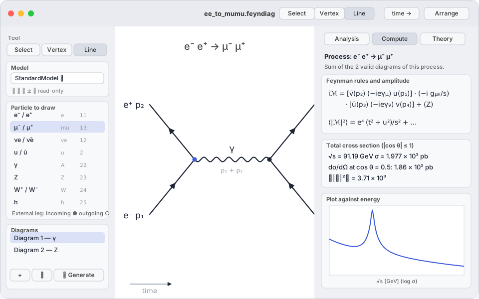
In a single window, TreeLevel chains together what usually takes a table of rules, a symbolic algebra program and an integration code.

The theory comes first
The full Standard Model (Feynman gauge, complex CKM), QED, φ⁴, an effective hadron model, minimal SU(5). Write your own in a small readable language, or import a UFO folder (MadGraph/FeynRules): the MSSM imports completely, 822 vertices.
Rules, derived
Every interaction term becomes a vertex: combinatorial factors, momenta, colour and Dirac structure. Nothing is copied from a table — the 129 Standard Model vertices agree one by one with MadGraph's.
Draw, check
Three tools are enough. The canvas reads the diagram along the time axis: a line running backwards in time is an antiparticle. The inspector tells you at once whether the diagram is consistent, and if not, why.
Sum the diagrams
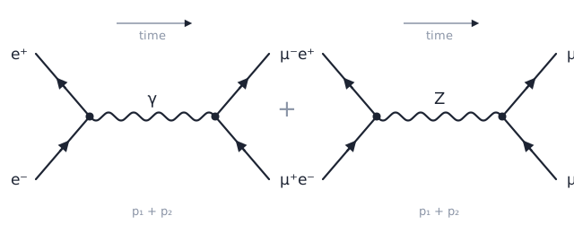
The Generate button enumerates every tree diagram of a process. The valid diagrams of one process are summed with their relative signs, Majorana fermions included.
Compute fast
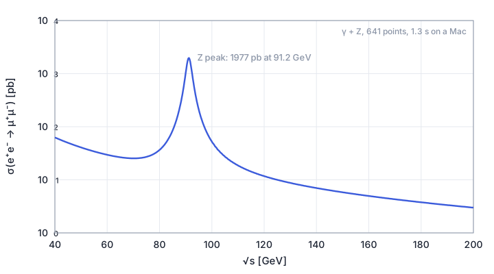
Numerical helicity amplitudes on all cores: a σ(√s) scan over 641 energies takes a second. Quadrature for 2 → 2, closed formulas for 1 → 2, Dalitz for 1 → 3, RAMBO Monte Carlo beyond.
And see the formula
The symbolic engine computes ⟨|ℳ|²⟩ in s, t, u with Dirac traces, polarisation sums and colour factors; rules and amplitude are displayed in LaTeX, and agree with the numerical result to 10⁻⁸.
What it looks like
| Quantity | TreeLevel | Reference |
|---|---|---|
| Muon lifetime | 2.19 µs | 2.197 µs (measured) |
| Z, W and Higgs widths (tree-level channels) | partial widths and branching ratios | Particle Data Group |
| Γ(π⁰ → γγ) (effective model, anomaly) | 7.79 eV | 7.7 eV |
| Neutron lifetime (tree level, gA = 1.27) | 946 s | 879 s (no radiative corrections) |
| e⁺e⁻ → W⁺W⁻ | gauge cancellation between γ, Z and ν | correct high-energy behaviour |
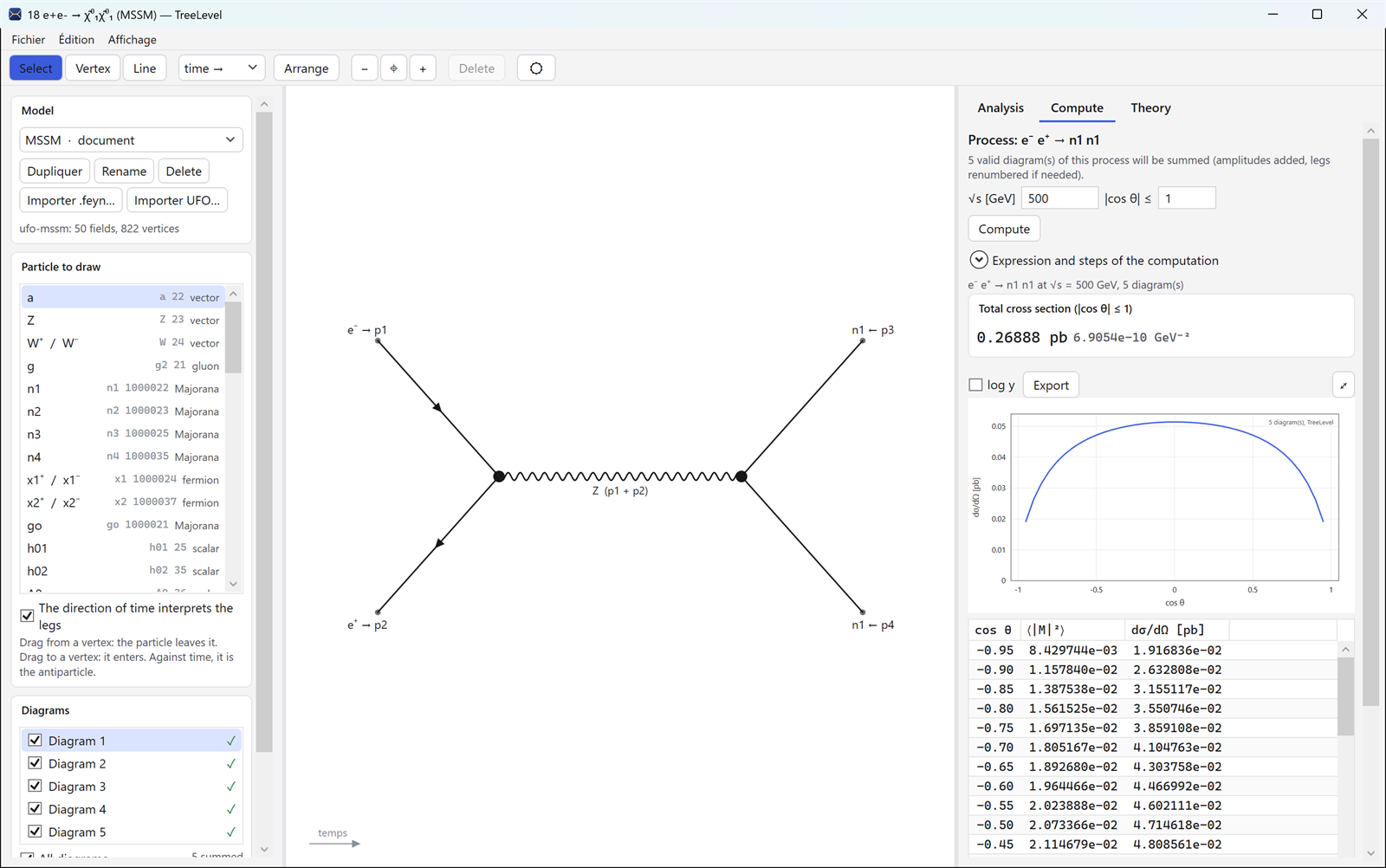
| σ(e⁺e⁻ → χ̃⁰₁χ̃⁰₁) at 500 GeV, MSSM SPS1a | 269 fb | 250–300 fb (ILC studies) |
| SU(5): branching ratios of X and Y | ½ ½ ; ½ ¼ ¼ | Georgi–Glashow |
On Windows too
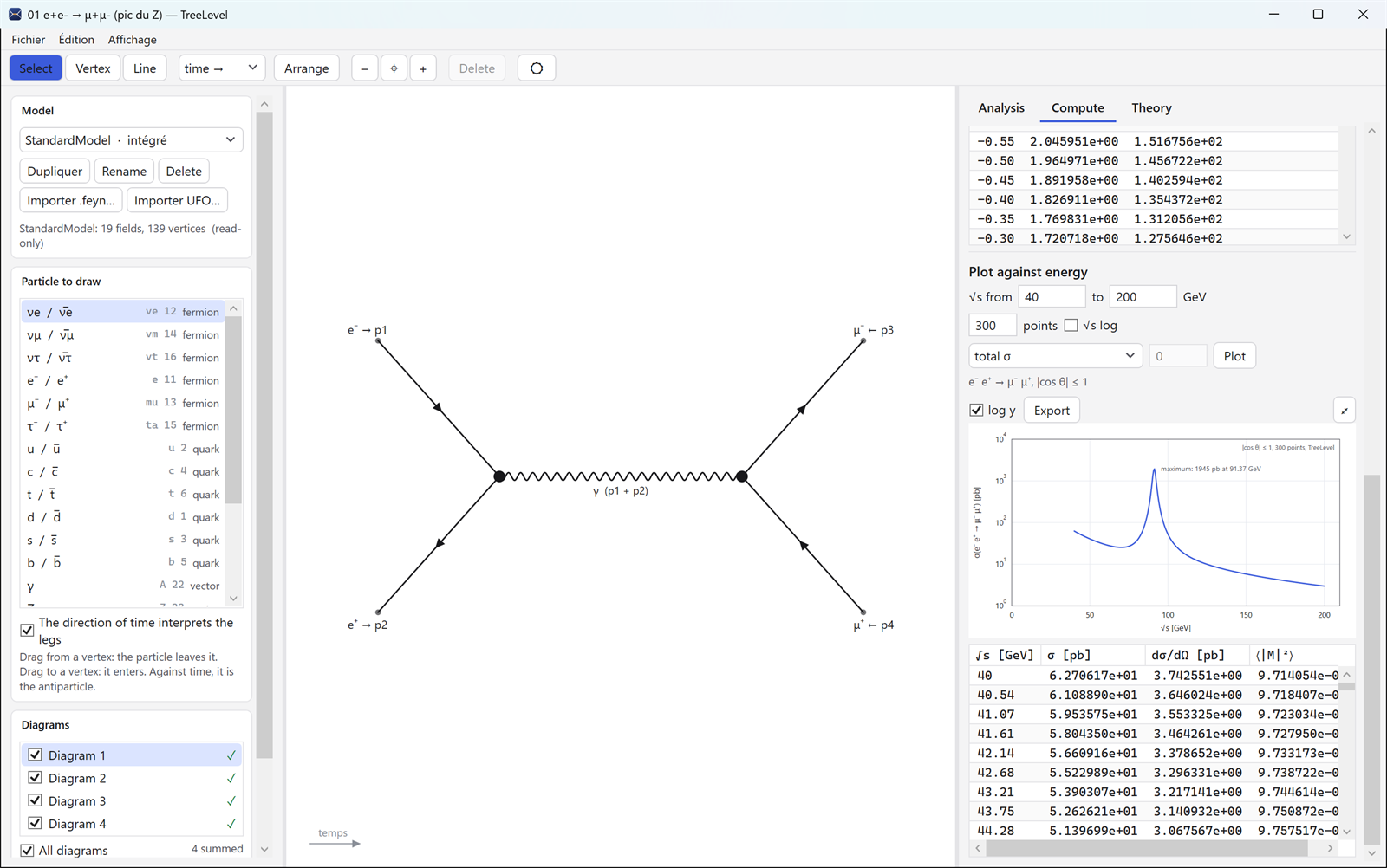
The same application on PC, Windows 10 and 11, x64 and ARM64: the same engine, the same .feyndiag documents interchangeable with the Mac, the same interface in 11 languages.
Who is it for?
For the student learning Feynman rules who wants to see, on their own diagram, what each vertex becomes; for the teacher preparing an exercise and its solution; for the physicist who needs a tree-level order of magnitude without launching a MadGraph chain, or who wants to check the rules of a model they have just written.
What TreeLevel does not do (yet). No loops, no parton distribution functions: cross sections are partonic or leptonic. Resonance widths enter the propagators, but radiative corrections do not. See the Physics page.