 TreeLevel
User manual
Everything TreeLevel does, panel by panel. To learn by doing, start with the tutorials instead.
The interface is available in English, French, German, Italian, Spanish, Portuguese, Russian, Chinese, Japanese, Korean and Hindi (following the system language). The French labels are given in parentheses where they differ in spelling, for readers of the French documentation.
The window
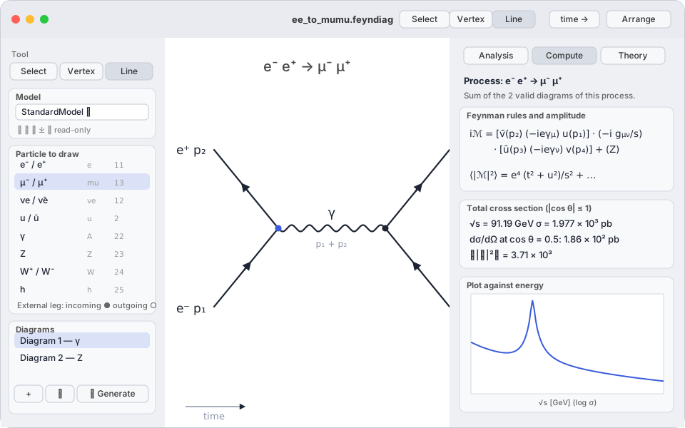
A TreeLevel document (.feyndiag) holds one theory and one set of diagrams for a process. The window has three areas:
- The palette: the tool, the model, the particle to draw, the list of the document's diagrams.
- The canvas: the current diagram. You place vertices, drag lines, and move everything with the mouse.
- The inspector, in three tabs: Analysis (Analyse — is the diagram valid, which rules, which amplitude), Compute (Calcul — ⟨|ℳ|²⟩, σ, Γ, τ, plots) and Theory (Théorie — the model's Lagrangian).
Choosing a theory
The Model (Modèle) box of the palette lists the built-in models, then My models (Mes modèles). Changing the model reloads the particle palette and invalidates the current analyses.
| Built-in model | Content |
|---|---|
StandardModel | The Standard Model in the broken phase, Feynman–'t Hooft gauge: 3 families, complex CKM, Higgs, Goldstones, gluons. 139 vertices. |
QED | Electrons and muons coupled to the photon. Ideal for first computations (Bhabha, Compton, annihilation). |
Phi4 | A real scalar and its −λ/4! φ⁴ coupling: the smallest possible model. |
Hadrons | Effective model of 32 fields, point-like hadrons (momentum transfers ≲ 0.5 GeV, no form factors): nucleons and hyperons Λ, Σ±,0, Ξ0,−; π, K, KS, KL, η, D, Ds, B; ρ⁰, ω, φ, J/ψ, ψ(2S), Υ; the three charged leptons and their neutrinos; γ, W, Z. Couplings: QED, charged and neutral currents of leptons and nucleons, decay constants fπ, fK, fD, fDs, fB (P → ℓν, τ → πν, Kν), f₊ (K → πℓν), anomaly (π⁰, η → γγ; ω → π⁰γ), ρ → ππ, φ → KK, vector mesons → ℓ⁺ℓ⁻ (fixed by Γee), hyperons → Nπ (S and P amplitudes fitted to Γ and α), semileptonic (f₁, g₁), Σ⁰ → Λγ (transition moment). Ω⁻ (spin 3/2) is absent. |
SU5 | The Standard Model plus the X (charge 4/3) and Y (1/3) gauge bosons of Georgi–Glashow: baryon and lepton number violation (B − L conserved). |
MajoranaTest | A heavy Majorana neutrino mixing with the electron: the simplest model with non-trivial fermion-flow rules. |
Built-in models are read-only. The buttons under the selector:
- Duplicate (⧉) copies the current model into My models, where it becomes editable in the Theory tab.
- Rename, Delete — for your own models only.
- Import a
.feynfile written by hand (see Theories). - Import a UFO folder (📁): a MadGraph/FeynRules model (SM, MSSM, …) becomes a library model with its vertices ready to use; the Theory tab shows the import notes.
Your models are kept in the application's container and remain available from one document to the next; the document itself embeds a copy of the theory, so it stays computable on another Mac.
Drawing a diagram
The canvas pans (drag the background with the Select tool), zooms (pinch on the trackpad, ± toolbar buttons, ⌘+ / ⌘−) and recentres on the diagram (⌘0 or the middle button); the zoom factor is shown bottom right. Three tools, in the toolbar as in the palette:
| Tool | Gesture | Effect |
|---|---|---|
| Vertex | click on the canvas | places a vertex. Dropped on the free end of a leg, it connects to it. |
| Line (Ligne) | drag from one vertex to another | internal line (propagator) of the particle selected in the palette. |
| drag from a vertex into empty space | external leg leaving the vertex. | |
| drag from empty space to a vertex | external leg entering the vertex. | |
| Select (Sélection) | click, drag | selects and moves a vertex or the end of a leg; the Selection box of the Analysis tab shows its properties. ⌫ or the Delete button removes it. |
The Particle to draw (Particule à tracer) box lists the model's fields with their display name (e⁻ / e⁺, W⁺ / W⁻ …), their name in the model language and their PDG Monte Carlo code. Hover over a particle: a tooltip recalls spin, charge, colour, mass and width.
Every external leg gets a number: it is its momentum p₁, p₂, … in the rules and the amplitude. Select a leg to change its particle (Field), switch it to the antiparticle, or fix its direction when the direction of time does not interpret it. Select an internal line to see its field and the direction in which the particle travels (from → to; Reverse the flow).
The direction of time
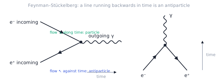
By default the option The direction of time interprets the legs (Le sens du temps interprète les pattes) is on. The canvas then reads the diagram as one reads it in a textbook: the position of a leg relative to its vertex along the time axis (time → or time ↑) makes it incoming or outgoing, and a fermion line whose arrow runs backwards in time is the antiparticle. While you drag a leg, the palette announces what it will be on release.
Switch the option off to set incoming / outgoing and particle / antiparticle yourself on each leg — useful for a diagram drawn in an unusual layout. The direction of time has no effect on the computation: it only acts on the reading and on Arrange, which puts the incoming legs on one side and the outgoing ones on the other.
Checking: the Analysis tab
The analysis is redone after every change. At the top: the process (for instance e⁻ e⁺ → μ⁻ μ⁺), the number of legs, vertices, internal lines and loops, then the verdict:
- Consistent diagram (Diagramme cohérent), with its symmetry factor and the number of fermion loops; or
- an error (the engine's messages are in English): a vertex has only two lines; the diagram is not connected — a leg ending near a vertex is not attached to it; or the vertex e ve W does not exist in this model, in which case the list of the model's vertices sharing most of these fields is given, to spot a forgotten antiparticle.
Then come the boxes Vertices (the rule attached to each vertex, its incoming momenta), Internal momenta (each propagator with its momentum in terms of the pi), Fermion chains (in which order the spinors are read — with Majorana fermions, the orientation of each chain), and Feynman rules and amplitude: the vertices in LaTeX and the assembled amplitude iℳ, spinor chains and propagators spelled out.
The analytic ⟨|ℳ|²⟩ box runs the symbolic engine on all the valid diagrams of the process: Dirac traces, polarisation and colour sums, initial-state average, result in s, t, u. Three checkboxes simplify the expression: massless particles omitted, u = Σm² − s − t, cW² = 1 − sW².
Several diagrams, generation
The Diagrams (Diagrammes) box holds the list of the document's diagrams. + adds an empty diagram, ⧉ duplicates the current one keeping its external legs (handy to draw the second diagram of the same process), − removes it. The checkbox in front of each diagram decides whether it enters the sum of amplitudes; All diagrams (Tous les diagrammes) checks or unchecks everything, and the counter “n summed” says how many will actually be summed. The choice is saved with the document — handy to isolate one channel (the Z alone, the t channel alone) or to measure an interference by comparing with and without.
Generate (Générer) enumerates every tree diagram of the process defined by the external legs of the current diagram, lays them out automatically and names them after their vertices and propagators. Two variants: Add the missing diagrams completes your drawings without touching them (duplicates are recognised whatever their layout); Replace by all tree diagrams starts over.
All the computations of the Compute tab bear on the sum of the amplitudes of the valid diagrams of the document that describe the same process as the current diagram — same incoming and outgoing particles, whatever the order in which you dragged the legs: the momentum labels pi are aligned automatically with those of the current diagram. The number of diagrams summed is recalled before each result, and the diagrams left out are listed with the reason (unchecked diagram, invalid diagram, or another process). To isolate the contribution of a single diagram, delete the others — or duplicate the document.
Computing: the Compute tab
For a 2 → 2 scattering: enter √s in GeV and cos θ (scattering angle in the centre of mass), then Compute (Calculer). You get ⟨|ℳ|²⟩ (averaged over initial spins and colours, summed over final ones), dσ/dΩ in pb at that angle, a table of dσ/dΩ(cos θ) and the total cross section integrated by Gauss–Legendre quadrature, with a cut |cos θ| ≤ c for processes with a Coulomb pole (Bhabha, low-energy Compton…) where the total σ diverges. The dσ/dΩ(cos θ) curve can be switched to a log y scale and exported (see below).
The Expression and steps of the computation group shows, during and after the computation, what the engine does: contracted tensor network, helicity loop, averaging factors, GeV⁻² → pb conversion (1 GeV⁻² = 0.3894 mb). Computations use all cores.
Plotting against energy
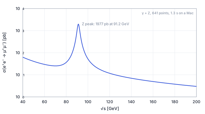
Plot against energy (Tracé en fonction de l'énergie): give √s from … to …, the number of points, log or linear scale, the Quantity (total σ, dσ/dΩ at a given cos θ, or ⟨|ℳ|²⟩), then Plot (Tracer). The axes fit the data; a resonance peak appears if the boson's width is declared in the model. The √s log checkbox spaces the points logarithmically (and puts the x axis on a log scale), the log y checkbox (ordonnée log) changes the vertical scale without recomputing.
A click on a chart (or on the magnifier) opens it enlarged in a resizable sheet, with the same settings and the same export menu. Every chart — the energy scan as well as the dσ/dΩ(cos θ) curve — has its Export (Exporter) menu: PNG image (double resolution), PDF document or SVG drawing (vector) — in a publication style: framed axes, grid, 10ⁿ ticks on log axes, annotated maximum — or CSV data (all the columns of the table), with a title recalling the process and the energy.
Decays
When the diagram has a single incoming leg, the Compute tab becomes that of a decay at rest: Partial width Γ (closed formula for two bodies, Dalitz integration for three), Lifetime τ = ħ/Γ and Half-life T½, and if the model declares a Total width for the parent particle, the Branching ratio.
τ and T½ assume that the summed diagrams make up the whole width. For the muon or the charged pion this is true; for the Z, use the branching ratio. Identical particles in the final state get their 1/n! factor automatically (X → u u, π⁰ → γγ, h → …).
Beyond 2 → 2: Monte Carlo
For 2 → 3, 2 → 4, 1 → 4…, phase space is integrated by Monte Carlo (RAMBO algorithm), with the requested number of points and Cuts: minimum energy of each final particle, minimum mass of each pair, maximum |cos θ| with respect to the beam. The result comes with its statistical error. Cuts are indispensable as soon as a massless photon or gluon is emitted (soft and collinear divergences).
The Theory tab
It shows the source of the current model: the interaction Lagrangian, the fields, the parameters and their values, then the expandable list of all derived vertices. For a built-in model, Duplicate to edit; for one of your models, edit and Apply — syntax errors are reported with their line, and the diagrams are re-analysed with the new rules. Export… writes the model to a .feyn file, to share or version.
For a model imported from a UFO, the tab recalls the origin, the number of fields, vertices and parameters, and the Import notes (skipped vertices, conventions). Its rules are not editable: modify the original FeynRules model and import again.
Documents and preferences
File › Open an example (Ouvrir un exemple) offers eighteen ready-made documents: Z peak, muon decay, e⁺e⁻ → W⁺W⁻, Bhabha, Compton, u ū → t t̄, hadrons (π⁰ → γγ, neutron, Λ, τ, J/ψ, e⁺e⁻ → π⁺π⁻), Majorana, SU(5), imported MSSM. They are read-only: at the first edit, macOS offers to save a copy.
A .feyndiag document is created, opened and saved like any macOS document (⌘N, ⌘O, ⌘S); it holds the theory and the diagrams. The preferences (TreeLevel › Settings…) set:
- Text size — applies to the panels, the canvas labels and the formulas.
- Appearance (Apparence) — System, Day or Night; the day/night button of the toolbar (sun / moon) cycles through these three states, its menu lets you pick directly.
- At launch — reopen the last document, ask, or open a new document.