PlatformVersion

Simulating a detector

What an apparatus would see of the event: tracks bent by the field, deposits in the calorimeters, jets, and the energy that is missing.

This workspace came with version 1.2.

Defining the detector

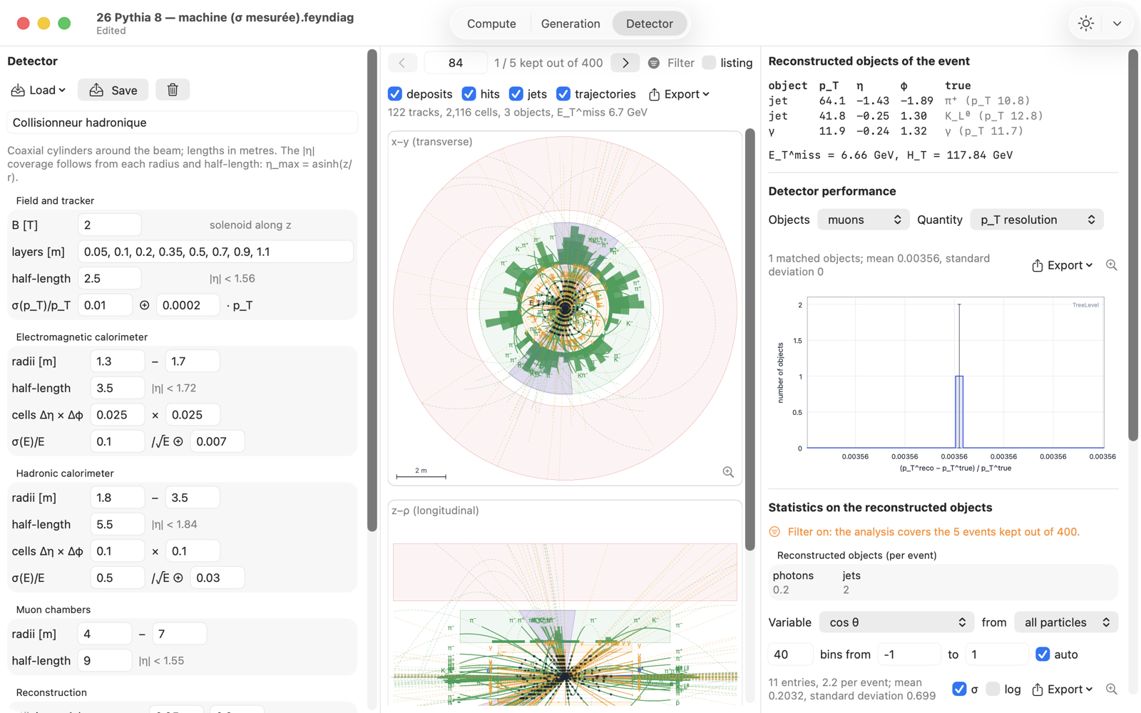
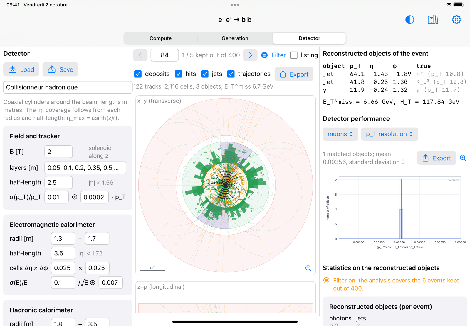
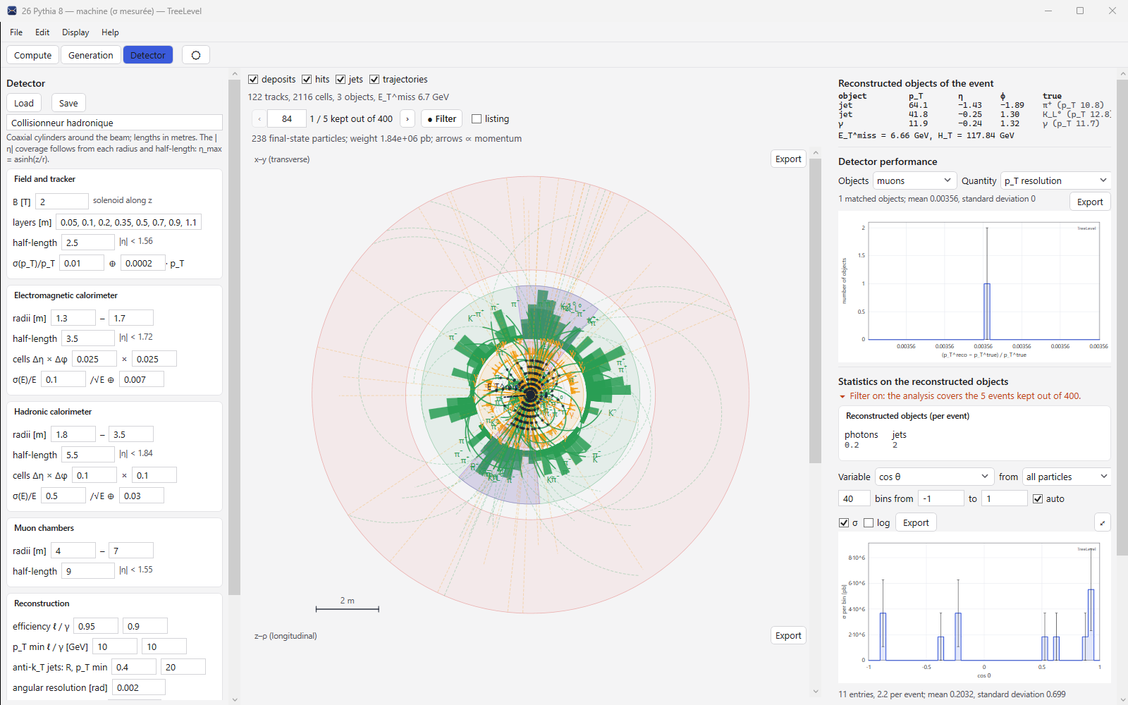
On the left, the detector definition: coaxial cylinders around the beam — tracker layers, electromagnetic and hadronic calorimeters (radii, half-length, $\Delta\eta\times\Delta\phi$ cells, resolution), muon chambers, solenoidal field — then efficiencies, thresholds, anti- $k_T$ jet parameters and the missing- $E_T$ resolution. Three presets (hadron collider, $e^+e^-$ , perfect); Save keeps your detector in “My detectors”, reusable in any document.

Endcaps close each barrel at both ends, as in ATLAS or CMS: three tracker discs, one disc per calorimeter, a wheel of muon chambers. Each sits right at the end of its barrel — 5 cm past it, so that the two can be told apart in the $z\text{–}\rho$ cut —, as wide as the barrel, and stops short of the next endcap; you set its thickness, and the radius of the beam hole, common to all. The $|\eta|$ coverage then reaches the hole — about 3.9 for the e.m. calorimeter of the hadron-collider preset, instead of 1.7 —, forward jets are reconstructed, and what escapes through the hole is missing from the missing- $E_T$ balance, as in a real experiment. A document made with an earlier version opens without endcaps and gives its results again. The endcaps of the calorimeters and muon chambers can also sit inside their barrel (in.): in its bore, flush with its end, the barrel wrapped around them; the tracker discs stay after its barrel.

The cross-sections and the objects

In the middle, the $x\text{–}y$ and $z\text{–}\rho$ cross-sections of the detector with the current event: helices of the charged particles in the field, hits on the layers, calorimeter deposits per cell, jets, missing $E_T$ . On the right, the reconstructed objects of the event, the detector performance on the sample ( $p_T$ and $\eta$ resolution, efficiency versus $p_T$ and $\eta$ , per object type) and the same statistics as in Generation, on the reconstructed objects.

TreeLevel's Detector workspace on the Mac: a proton-proton collision at 13 TeV in the x–y and z–ρ cuts, with its tracks, deposits and reconstructed jets — The Detector on a 13 TeV proton-proton collision (Machine source, Pythia 8): 122 tracks curling in the field, more than 2,000 cells hit, two jets and a photon reconstructed.

TreeLevel's Detector workspace on the iPad: a proton-proton collision at 13 TeV in the x–y and z–ρ cuts, with its tracks, deposits and reconstructed jets — The Detector on a 13 TeV proton-proton collision (Machine source, Pythia 8): 122 tracks curling in the field, more than 2,000 cells hit, two jets and a photon reconstructed.

TreeLevel's Detector workspace on Windows: a proton-proton collision at 13 TeV in the x–y and z–ρ cuts, with its tracks, deposits and reconstructed jets — The Detector on a 13 TeV proton-proton collision (Machine source, Pythia 8): 122 tracks curling in the field, more than 2,000 cells hit, two jets and a photon reconstructed.

The 3D view

Below the two cuts, the 3D view shows the detector in volume, at three quarters: the barrels and endcaps as a lightly shaded wireframe, the helices in the field, the hits. A click enlarges it; drag to turn it, pinch or use the wheel to zoom, and scroll to move it; a double-click brings back the starting view.use the wheel to zoom; a double-click brings back the starting view.pinch to zoom; a double tap brings back the starting view. The Show menu chooses what you see — each part of the detector, the endcaps, the trajectories, the hits, the jets (a faintly tinted cone), the deposits (as towers): overlapping transparencies soon become unreadable, so you keep only what you are looking at. By default: the tracker, the e.m. calorimeter, the endcaps, the incoming particles, the trajectories, the hits and, at the femtometre, the strings.

The enlarged cross-section: zoom, scale, vertex

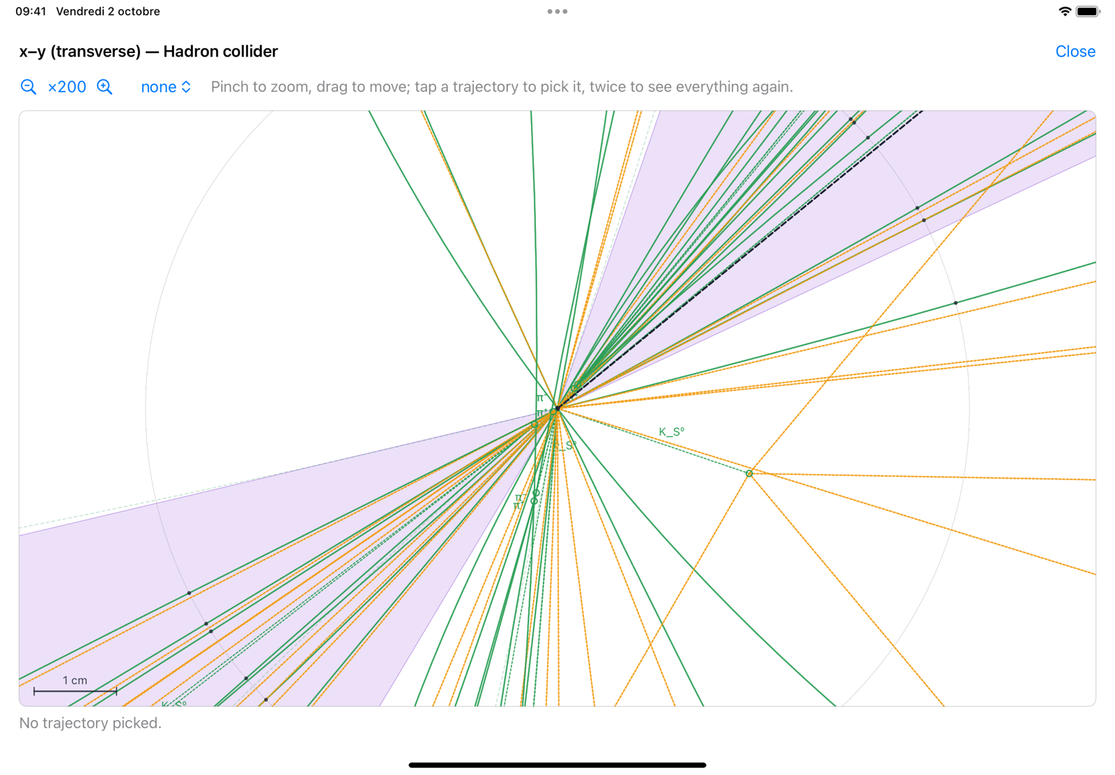
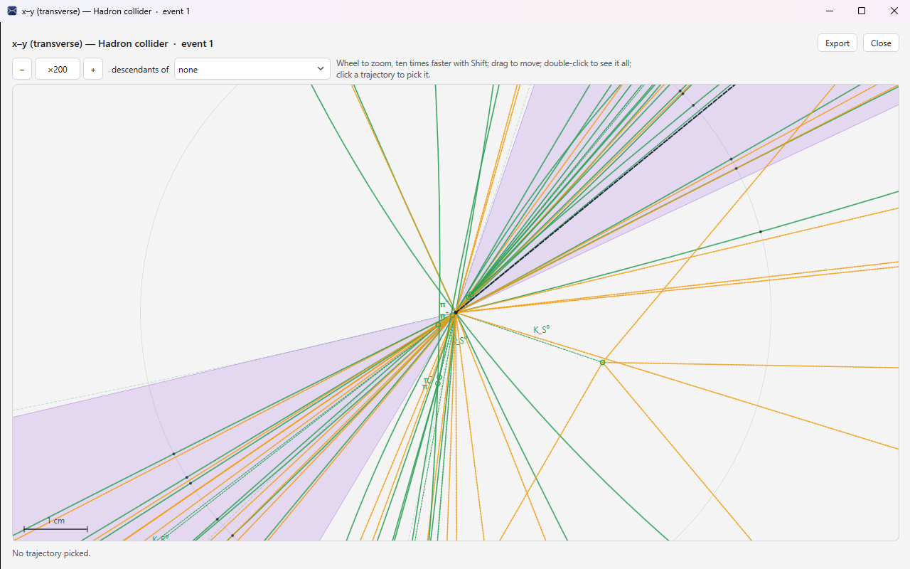
A click on a cross-section opens it in its own resizable window, which follows the current event; Esc or the ⓧClose button closes it. There you can zoom in up to a trillion $10^{16}$ times, from the metre of the detector down to the femtometre:

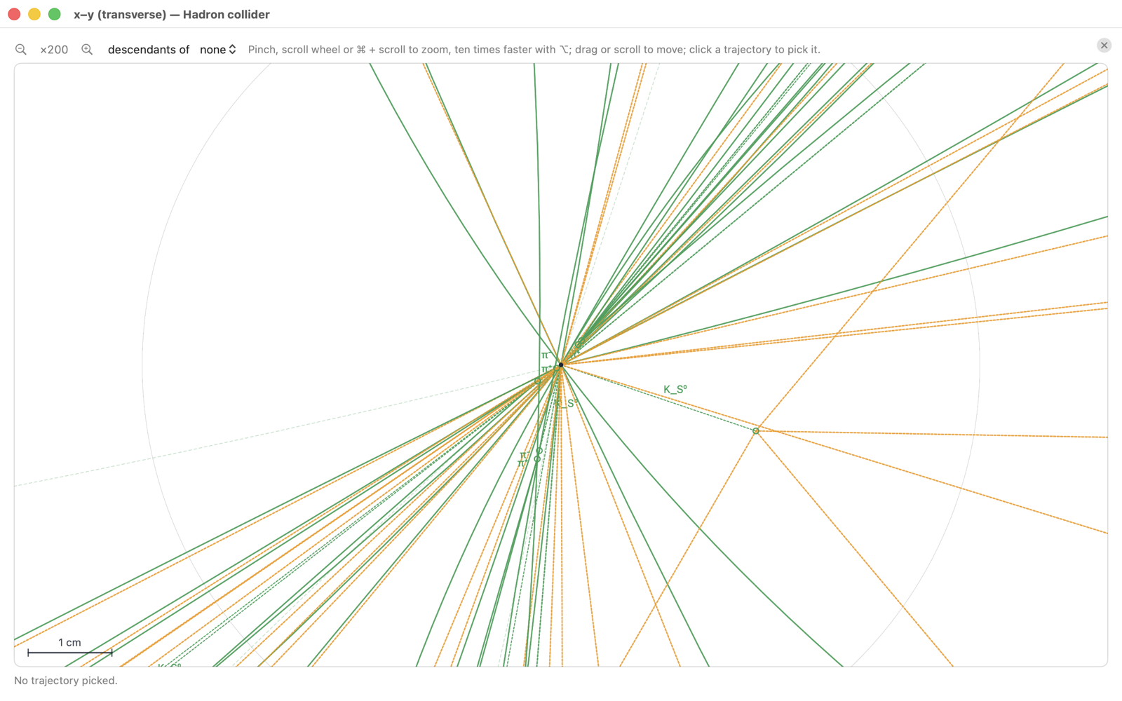
The enlarged cut at ×200 around the interaction point, with a one-centimetre scale bar — The enlarged cut, ×200 around the interaction point: a $K^0_S$ flies some 2.5 cm before decaying; the scale bar is 1 cm long.

zoom: pinch on the trackpad, one notch of the scroll wheel, ⌘ + scroll, ⌘+ and ⌘−; with ⌥, ten times faster. The zoom is centred on the pointer;
zoom: one notch of the scroll wheel, Ctrl + and Ctrl −; with Shift, ten times faster. The wheel zooms around the pointer;
zoom: pinch, or the − and + buttons above the cut; the zoom centres on your fingers;
move: drag, or scroll on the trackpad; see it whole: double-click or ⌘0;
move: drag; see it whole: double-click or Ctrl 0;
move: drag with one finger; see it all again: double-tap;
the grid box lays a light grid whose mesh is the length of the scale bar, and follows it as you zoom;
the Show menu chooses the parts of the detector and of the event — by default everything but the deposits. The incoming particles come from the edge along the beam to the collision; the $x\text{–}y$ cross-section, which sees them head-on, marks them at the vertex: ⊙ the one coming towards you, ⊗ the one moving away;
a scale bar, at the bottom, tells what a length stands for — 1 m, 5 cm, 200 µm, 10 nm, 1 fm.

Trajectories start from their production vertex, the one the generator computed. The primary vertex is a filled dot, a decay vertex a hollow one, and the mother that flew there is drawn: solid if charged, dotted if neutral. You can see the V's of $K^0_S$ and $\Lambda$ a few centimetres out, B's at the millimetre, the $\tau$ at under a hundred micrometres. As soon as ten micrometres can be read on screen, a banner warns that you are looking finer than a silicon tracker can locate; at the femtometre, that the positions are those of the hadronisation model.

Hovering over a trajectory tells what it is. A click picks it: it turns bold, with $p_T$ , $\eta$ , $\phi$ , its vertex, where it decayed and after what distance, its impact parameter $d_0$ , its lineage back to the hard process and its line in the listing. The descendants of menu brings out everything a particle gave — the jets of a W, the leptons of a Z, the products of a B —, and the rest fades. Hadrons are named: B, D, $\Lambda_b$ , $\Lambda_c$ , and the others.

The filter of the Generation workspace works here too, on what the detector reconstructs — see Filtering the events.

The interaction zone

At the femtometre, the enlarged cross-section shows the zone where the collision took place, as the generator models it: nothing seen there is measured. For Pythia 8 to place the particles there, tick positions in the interaction zone (model, fm) in the settings of the Generation workspace — the box appears once TreeLevel Tools 0.5the Pythia module 0.5 or later is installed. The partons and strings (model) layer of the Show menu then draws:

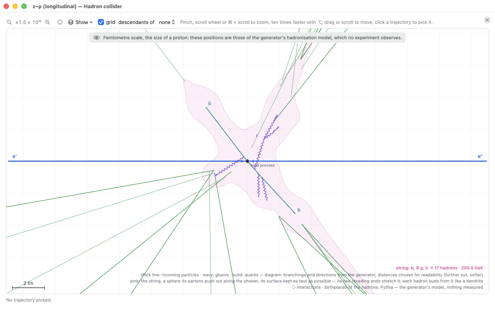
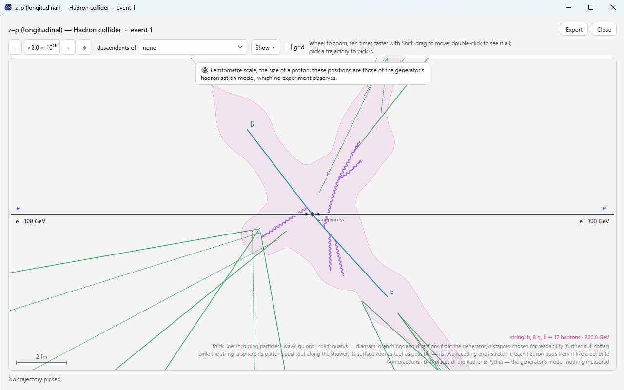
The z–ρ cross-section ×2·10¹⁵ of an e⁺e⁻ → b b̄ annihilation at 200 GeV, with the pink body of the string — The interaction zone of an $e^+e^-\to b\bar b$ annihilation at 200 GeV, $\times2\cdot10^{15}$ : the body of the string, stretched between the receding $b$ and $\bar b$ , pulled by its gluons; the hadrons leave from it. The scale bar measures 2 fm.

the incoming particles, in a thick line, coming from the beam; a diamond marks the hard process and each multiple interaction;
the shower: each parton leaves in the direction of its momentum — wavy gluons, solid quarks —, the hard branchings near the centre, the soft ones further out. The branchings and the directions are the generator's; the distances are chosen for readability;
the body of each colour string, in pink: a sphere at the vertex that its partons push out along the shower, its surface kept as taut as possible; its two ends, moving apart, stretch it. Each hadron buds from it like a dendrite tapering to the point where Pythia has it born, and its trajectory starts there. A hadron born very far away — thousands of femtometres along the beam, in a proton collision — is joined to it by a filament.

Read this first. The shower, the strings and the dendrites are neither a measurement nor a prediction: they are a graphical, heuristic reconstruction of the simulation, more artistic than scientific, of processes that have no rigorous counterpart. Only the interaction vertices and the birthplaces of the hadrons come from the generator — and they are themselves the positions of its model, which no experiment observes. This view illustrates; it does not claim to represent reality.

The legend describes each string of the hard process: its partons, its hadrons, its mass. The crosshair button ⌖ (⌘⇧0Ctrl Shift 0) brings the collision back to the centre without changing the zoom, and the view then follows it from one event to the next. The 3D view shows the same body in volume, shaded, when you come close to it, with the partons and strings (model) layer ticked in its Show menu.