Tutorials

Four walks, from the first diagram to physics beyond the Standard Model. Each takes about ten minutes; the numbers quoted are those TreeLevel displays. The interface follows the system language; the labels used below are the English ones.

1. $e^+e^-\to\mu^+\mu^-$: a first computation, then the Z peak

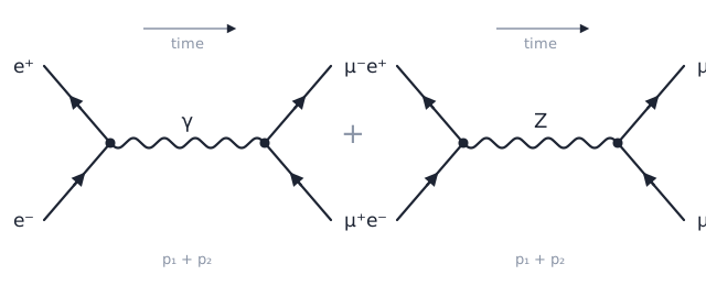
1. New document (⌘NCtrl Nthe browser's Create Document button). In the palette the StandardModel is selected; leave the direction of time on time →.
2. Vertex tool: click twice on the canvas, left and right, to place two vertices.
3. Line tool, particle $\gamma$: drag from the left vertex to the right one. That is the photon propagator.
4. Particle $e^-/e^+$: drag from empty space, bottom left, to the left vertex — the palette announces that an $e^-$ enters. Repeat from the top left: the fermion-flow arrow will run backwards in time, the leg is read as an incoming $e^+$. (The order in which you drag the two legs does not matter: what counts is the direction of the arrow.)
5. Particle $\mu^-/\mu^+$: drag from the right vertex into empty space, top right (outgoing $\mu^-$), then from empty space at the bottom right to the vertex (the arrow comes back to the vertex: outgoing $\mu^+$).
6. Look at the Analysis tab: Process: $e^-e^+\to\mu^-\mu^+$, consistent diagram. If the analysis reports a non-existent vertex, one of the legs is read the wrong way: select it and tick Antiparticle, or move its end to the other side of the vertex.
7. Expand Feynman rules and amplitude: the vertex $-ie\gamma^\mu$ twice, the propagator $-ig_{\mu\nu}/(p_1+p_2)^2$, the spinors $\bar v(p_2)\ldots u(p_1)$ and $\bar u(p_3)\ldots v(p_4)$.
8. Compute tab: $\sqrt s = 40\ \mathrm{GeV}$, Compute. $\sigma = 62.3\ \mathrm{pb}$. Check by hand: $\sigma = 4\pi\alpha^2/3s$ with $\alpha = 1/127.9$ (the model's value at $M_Z$) and $1\ \mathrm{GeV^{-2}} = 3.894\times10^8\ \mathrm{pb}$ gives $62.3\ \mathrm{pb}$.
9. Back in the palette, click Generate › Add the missing diagrams: the Z diagram appears — together with h and $G^0$ exchange, proportional to $m_e$ and negligible (the No scalar exchange option of the Generate menu avoids them). The computation now bears on the sum.
10. Plot against energy: from 40 to 200 GeV, 300 points, log scale, Plot. The Z peak reaches $1{,}979\ \mathrm{pb}$ at $\sqrt s = M_Z = 91.19\ \mathrm{GeV}$, with the width $\Gamma_Z = 2.495\ \mathrm{GeV}$ declared in the model. The curve goes through a minimum near $70\ \mathrm{GeV}$ ($25\ \mathrm{pb}$) before rising towards the resonance; the $\gamma$–Z interference, proportional to the small vector couplings $g_V$, stays discreet in the total $\sigma$ — it shows up in the forward–backward asymmetry.

2. The muon lifetime

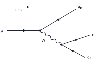
1. New document, model StandardModel. Place two vertices.
2. Line $W^+/W^-$ between the two vertices: a virtual W.
3. Particle $\mu^-/\mu^+$: drag from empty space, on the left, to the first vertex (incoming $\mu^-$). Particle $\nu_\mu$: drag from the first vertex into empty space (outgoing $\nu_\mu$).
4. At the second vertex: outgoing $e^-$ (from the vertex into empty space) and outgoing $\bar\nu_e$ — drag the leg from empty space to the vertex so that the arrow runs backwards in time.
5. Check in Analysis: $\mu^-\to\nu_\mu e^-\bar\nu_e$, consistent. A classic mistake is to draw the $\bar\nu_e$ as a particle: the requested vertex ve e W~ does not exist, and the inspector lists the neighbouring vertices that do (ve~ e W, e~ ve W~) — in other words, one leg must be reversed.
6. Compute tab: the decay is three-body, phase space is integrated exactly (Dalitz). $\Gamma = 3.007\times10^{-19}\ \mathrm{GeV}$, $\tau = 2.19\ \mu\mathrm s$, $T_{1/2} = 1.52\ \mu\mathrm s$. The measured value is $2.197\ \mu\mathrm s$; the difference is due to radiative corrections, absent at tree level.

Variant: in the Hadrons model, draw $n\to pe^-\bar\nu_e$ by W exchange ($\tau = 946\ \mathrm s$ at tree level with $g_A = 1.27$, against $879\ \mathrm s$ measured) or $\pi^+\to\mu^+\nu_\mu$, which has a single contact vertex.

3. $e^+e^-\to W^+W^-$: generate, sum, and see the gauge cancellation

1. New document. Place two vertices, drag the external legs: incoming $e^-$ and $e^+$ on the left, outgoing $W^-$ and $W^+$ on the right (particle $W^+/W^-$: dragged from the vertex into empty space the line is an outgoing $W^+$; from empty space to the vertex, i.e. against time, an outgoing $W^-$). Do not draw an internal line yet.
2. Generate › Replace by all tree diagrams: four diagrams — $\gamma$, Z and h exchange (negligible, $\propto m_e$) and $t$-channel $\nu_e$ exchange.
3. Compute tab, $\sqrt s = 200\ \mathrm{GeV}$: $\sigma = 19.2\ \mathrm{pb}$, as at LEP ($17\ \mathrm{pb}$ measured, radiative corrections included).
4. Delete the neutrino diagram (select it in the list, −) and recompute: $18.1\ \mathrm{pb}$. Almost nothing changes… at $200\ \mathrm{GeV}$.
5. Plot against energy, from 170 to 1,000 GeV, log scale: without the neutrino $\sigma$ grows ($118\ \mathrm{pb}$ at $500\ \mathrm{GeV}$, $385\ \mathrm{pb}$ at $1\ \mathrm{TeV}$); with the four diagrams it falls as it should ($7.1\ \mathrm{pb}$ at $500\ \mathrm{GeV}$, $2.4\ \mathrm{pb}$ at $1\ \mathrm{TeV}$). That is the cancellation between the gauge diagrams, and the reason for the triple-boson couplings of the Standard Model.

4. Beyond the Standard Model: SU(5) and the MSSM

SU(5): a boson that turns quarks into leptons

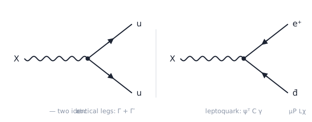
1. Choose the SU5 model. The palette gains two bosons, X (charge $4/3$) and Y ($1/3$), colour triplets of mass $10^{15}\ \mathrm{GeV}$.
2. Draw $X\to uu$: one vertex, incoming X, two outgoing u. Analysis: consistent, with the colour factor $\varepsilon_{abc}$ in the rule — a vertex that violates baryon number.
3. Compute: $\Gamma(X\to uu) = 4.17\times10^{12}\ \mathrm{GeV}$. Draw $X\to e^+\bar d$: the same width. The branching ratios $\tfrac12/\tfrac12$ are those of Georgi–Glashow; for Y you will find $\tfrac12\ (ud),\ \tfrac14\ (e^+\bar u),\ \tfrac14\ (\bar\nu\bar d)$, and $\Gamma_Y = \Gamma_X$, as befits two members of the same doublet.
4. Draw $uu\to e^+\bar d$ and generate: three diagrams ($s$-channel X, $t$- and $u$-channel Y). At $\sqrt s = 2\times10^{15}\ \mathrm{GeV}$, $\sigma = 7\times10^{-26}\ \mathrm{pb}$; the Analysis tab gives the full symbolic expression in $s, t, M_X, M_Y$.

The model file (Theory tab) shows how these couplings are written: bilinears $\psi^TC\gamma^\mu P_L\chi$ with the charge-conjugation matrix $C$. See the Theories page.

MSSM: importing a UFO

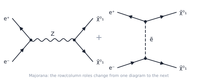
1. Download the MSSM_SLHA2 UFO folder from the FeynRules model database (or any UFO model shipped with MadGraph). In the palette, button 📁 Import a UFO folder, choose the folder.
2. A second later: “UFO imported: 50 fields, 822 vertices”. The model appears in My models; the palette lists neutralinos, charginos, squarks, sleptons and the gluino with their PDG codes (1000022 for $\tilde\chi^0_1$…).
3. Draw $e^-e^+\to\tilde\chi^0_1\tilde\chi^0_1$ (two outgoing n1 legs; the neutralino is Majorana, there is no antiparticle), then Generate: $s$-channel Z exchange, $t$- and $u$-channel $\tilde e_L$ and $\tilde e_R$ exchange.
4. Compute at $\sqrt s = 500\ \mathrm{GeV}$: $\sigma = 269\ \mathrm{fb}$ at the SPS1a point, within the range of the linear-collider studies. The row/column roles of the external spinors change from one diagram to the next: TreeLevel applies Denner's fermion-flow rules, and the result does not depend on the chosen orientation.